

Financial Statement Fraud Detection Machine Learning Model Design
We propose designing a financial statement fraud detection machine learning model in this study. The model is a classification algorithm chosen among several tested in this study. The decision tree has given better precision compared to others. The main features were based on the conjunction of two proven mathematic empirical models, Beneish M-Score and Altman Z-Score. Both models were combined to give one new model. It is proven that each model separately can detect fraud with at least 90% accuracy.
Research question: How to design a machine learning classification using Beinish M-Score and Altman Z-score?
Introduction
Financial reporting is a mandatory document for any company; different parties use it for diverse goals. Investors can evaluate the financial health of a firm before investing. The government uses it for tax purposes. Stakeholders can use it for financial analysis. False reporting misleads all analysis and interpretation of financial reporting with severe consequences. Some well-known scandals, such as the Waste Management Scandal in 1998, the Eron Corp scandal in 2001, and the Worldcom scandal, resulted in billions of dollars in losses and bankruptcy. Many models to detect financial distress have been developed. Among them, this study focuses on two models: Beinish M-Score [1] and the Altman Z-Score model [2]. These models are mathematically probabilistic. (Altman et al., 2010) [2]. It Showed that the model was accurate, with a correct prediction percentage of about 95%, and received many positive reactions.
Beinish (1999) [1] correctly predicted 76% of financial distress while incorrectly indicating 17.5% of non-financial distress.
Both Beinish M-Score and Altman Z-Score models are based on empirical mathematical formulas, and the limit zone of decision is constant, which is good when evaluating only one company once. Generally, a single mathematical formula is applied to one element only and not to a dataset, so if the variable environment changes, the formula will not dynamically catch the change. In our study of financial reporting fraud behavior, we deal with a very dynamic economic environment, so that some macroeconomic change can affect the trade between companies, or a financial crisis can affect the industry with a relative impact per sector. This situation can systematically falsify the results when using these static empirical models. Thus, using industry performance as a benchmark and adapting the zone limit decision, which was constant for a single company, can now be variable when evaluating one company concerning another company’s performance. This approach is more realistic and allows us to make better decisions.
Muntari (2015) [3], during his study of the Eron Corp scandal, used both Altman Z-Score and Beinish M-Score to evaluate the Eron Corp financial manipulation, got a contradiction in the year 1999, when the result showed for Alman Z-Score a value of 3.040 and Beinish M-Score a value of -1.323. This situation makes Eron Corp good considering the Altman Z-Score decision and bad for Beinish M-Score. This contradiction cannot be solved by lecturing both models separately using their constant limit zone of decision. In this study, we propose to solve this situation with a data-driven model that uses industry performance to make decisions.
Combining both model types and building one that detects the different zones based on the industry’s behavior. If the binary classification is studied, then the distress zone is not roughly determined by the mean of the empirical mathematical formula, which is more of a determinist approach, but rather by learning from other companies’ data and then classifying the studied company. A correlation study can determine a combined model based on the two models.
This study is structured with the following points:
- Data analysis to help build study assumptions
- Engineering data-driven models with various assumptions and features
- Machine learning binary classification compares the outcomes of different classification algorithms.
Empirical model M-Score and Z-Score Overview
ALTMAN Z-Score Context
Altman‘s Z-Score is a model used to predict whether a company is in financial distress.
The Altman Z-score is based on five financial ratios calculated from a financial statement report. It uses profitability, leverage, liquidity, solvency, and activity to predict whether a company has a high probability of being insolvent.
Muntari Mahama [3] shows that Z-Score can predict financial distress with 95% accuracy. He also demonstrated that the model could detect financial distress in the early stages of the Eron fraud scandal in 1997, before the bankruptcy in 2001. The Z-Score model confirmed the correlation between corporate governance and corporate failure.
ALTMAN Z-Score Mathematical Model
Z-Score [2] is done by the following formula: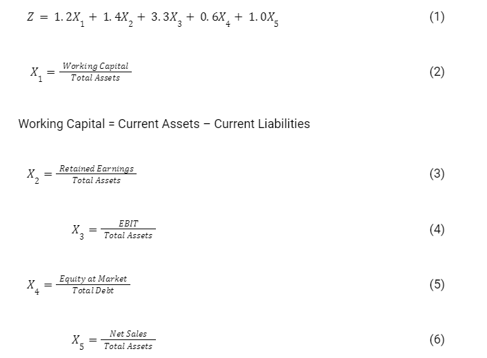
The interpretation of the Z-score is given below:
- Z ˃ 2.67 : interval free of distress
- 1.81 ˂ Z ˂ 2.67 interval warning of distress
- Z ˂ 1.81 interval of distress
Beinish M-Score Context
According to Muntari [3] and Ganga et al. [4], M-Score is a mathematical model that employs some financial metrics to determine the extent of a company’s earnings. The M-Score is like the Z-Score, except the M-Score concentrates on estimating the extent of earnings manipulation instead of determining when a company becomes bankrupt. The M-Score is composed of eight ratios that capture either financial statement distortions that can result from earnings manipulation or indicate a predisposition to engage in earnings manipulation, showing that M-Score can detect financial manipulation accurately. He also demonstrated that the model could detect financial manipulation in the Eron fraud scandal in the early stages of 1997.
Beinish M-Score Mathematical Model
The following mathematical expression gives the Beneish model [1]:
DSRI: Days’ sale in receivables index.
The index measures the ratio of days that sales are in accounts receivable in a year compared to that of the prior year. A value greater than 1.0 indicates possible revenue inflation.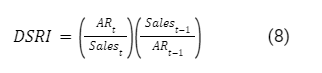
Where AR is Account Receivable
GMI: Gross Margin Index.
The gross margin index measures the prior year ‘s gross margin ratio with the one under review. A value greater than 1.0 indicates that the gross margin has worsened in the period under review. It indicates the possibility of revenue manipulation.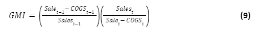
Where COGS is Cost of Goods Sold
AQI: The index indicates the change in asset realization risk by comparing current assets and property, plant, and equipment with total assets.
When AQI value is greater than 1.0, the company has potentially increased its cost deferral or increased its intangible assets and created earnings manipulation.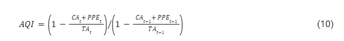
Where CA is the Current Assets, PPE is the Plant Property, and equipment TA is the Total Assets.
DSRI: This index measures the growth in revenue in one year over the prior year’s revenue.
If the value exceeds 1.0, it indicates positive growth, while less than 1.0 indicates negative growth in the year under review. Though other factors may be responsible, growth in sales may be interpreted to mean earnings manipulation.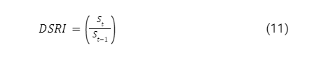
Where S is Sales
DEPI: This index measures the ratio of depreciation expense and gross value of PPE in one year over a prior year.
An index value greater than 1.0 could reflect an upward adjustment in the useful life of PPE. This can potentially to manipulate a company’s earnings in the current fiscal year.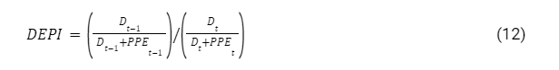
Where D is Depreciation expense and PPE is the Property Plant Equipment
SGAI: Sales, General, and Administrative Expenses Index.
This index measures the ratio of sales, general and administrative expenses to sales in one year over a prior year. A disproportionate increase in sales, as compared to SGAI, would serve as a negative indication concerning a company‘s future prospects.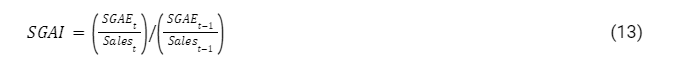
Where: SGAE: Sales, General and Administrative Expenses, S is Sales
TATA: Total Accruals to Total Assets.
The index assesses the extent to which management employs discretionary accounting policies that result in earnings.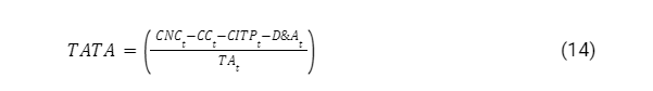
Where CNC Change in Working Capital, CC Change In Cash, CITP Change In Income Tax Payable, D&A Depreciation & Amortization, TA Total Assets
LEVI: The leverage index measures the ratio of total debt to total assets.
An index greater than 1.0 can be interpreted as an increase in the company’s gearing and, for that matter, exposed to manipulation.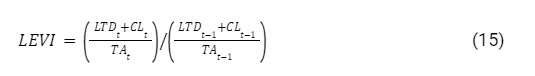
Where: CL Current Liabilities, TA: Total Assets, LTD Long Term Debt
Input Data Sample
Table 1: Sample of calculated score for 4 years
| 2015201620172018tickerAltman Z-ScoreBeinish M-ScoreAltman Z-ScoreBeinish M-ScoreAltman Z-ScoreBeinish M-ScoreAltman Z-ScoreBeinish M-ScoreAAPL4.998-2.8464.407-2.7523.652-2.5293.484-2.495ACIW2.376-2.8892.962-2.2882.803-2.6023.184-1.938ADI14.156-2.57110.723-3.1872.796-2.0533.393-2.671ADP2.350-1.8751.817-2.8562.177-2.8552.112-2.499ADSK8.940-2.7816.048-2.2734.901-3.8653.846-2.712AMAT5.240-2.1325.674-2.2465.057-3.4885.363-2.386AMKR0.465-3.2000.708-2.9060.797-3.0900.814-2.736ASGN2.639-2.3563.006-2.4713.373-2.3492.116-2.173AVGO13.501-2.7282.3410.6682.570-2.6693.915-2.612COMM0.552-2.2650.827-2.7130.872-2.6630.938-2.805CSCO3.802-2.5293.643-2.5543.369-2.6632.978-2.541 |
Figure 1: Beinish and Altman Score of all years in data set

The raw plot of all year shows similar behavior each year. Therefore only one year is sufficient for our study since we do not need trend analysis. In the remaining of the study, we are going to use only the year 2015.
Figure 2: Beinish and Altman Score of year 2015

There is no visual correlation between Beinish M-Score and Altman Z-Score.
Machine Learning Model Designing
We analyze basis statistics to make assumptions for a model and visualize some results. Only one year of data is necessary for our analysis. Other years can be used for the validation of the model. The Alman’s Z-Score outcome is a value from an empiric mathematical formula and the Beneish M-Score, so the range values of fraud evaluation are given below.
Table 2: Z-Score and M-Score Range
| Safe Zone (green) | Intermediate Zone (yellow) | distress Zone (red) | |
| Altman’s Z-Score | Z ˃= 2.99 | 1.81 ˂= Z ˂ 2.99 | Z ˂ 1.81 |
| Beneish M-Score | M <= -2.22 | -2.22 <M <= -1.78 | M > -1.78 |
Basic Statistics
Table 3: Basic statistics for year 2015
| Altman Z-Score | Beinish M-Score | |
| count | 27 | 27 |
| mean | 5.371 | -2.517 |
| std | 5.482 | 0.669 |
| min | -0.397 | -3.593 |
| 25% | 2.323 | -2.839 |
| 50% | 3.533 | -2.622 |
| 75% | 6.209 | -2.239 |
| max | 19.952 | 0.119 |
The general overview of this statistic seems normal, with more than 50% of each score being in the green zone. This means we assume that, in reality, most of companies are not engaging in financial statement manipulation. For this sample, Altman Z-Score’s mean is greater than 2.99, Beinish M-Score’s mean is lower than -2.22, and all 50% are in the green zone. These observations suggest that we assume that the mean can be used as a benchmark to evaluate a company’s financial distress compared to others in its industry.
Feature engineering
Features are selected to build the model that the classification algorithm will learn to achieve the expected results. The proper selection will lead to the final labels, which the classifier will use to train and test the model.
The first features calculated are the Altman Z-Score and Bernish M-Score, calculated from the formulas above. Let’s assign a variable name to each feature:
Altman calculated Z. Z-Score and M: derived from the Beinish M-Score, and D is the decision variable, and the feature selection aims to give D one of two values: true (1) or false (0), based on the model assuming that we will develop in the subsequent development. The issue is one of binary classification. The company is classified as financial fraudulent when D = 0 and not financial fraudulent when D = 1.
Let’s create small z and m, two variables value of Z and M, define the first decision path and handle the problematic case using data-driven assumptions and thus make a decision value. All features are dependent variables of Z and M, and all created features are independent of each other for a single company.
Table 3: First step of features selection
| Feature | Z : zone | M : zone | Value | Comment |
| F1 | Z[z ˃= 2.99] | M[m<= -2.22 ] | 1 | Both models converge to the green zone |
| F2 | Z[z ˂ 1.81] | M[m > -1.78] | 0 | Both models converge to the red zone |
| F3 | Z[1.81˂= z˂ 2.99] | M[-2.22 <m<= -1.78] | 0 | We assume if both converge in yellow zone they are distressed |
| F4 | Z[z ˃= 2.99] | M[-2.22 <m<= -1.78] | ? | Probematic case need to look the industry for decison |
| F5 | Z[z ˃= 2.99] | M[m > -1.78] | ? | Probematic case need to look the industry for decison |
| F6 | Z[1.81˂= z˂ 2.99] | M[m<= -2.22 ] | ? | Probematic case need to look the industry for decision |
| F7 | Z[z ˂ 1.81] | M[m<= -2.22 ] | ? | Probematic case need to look the industry for decision |
F4 to F7 are made to address the contradiction between M and Z. Both Z and M have a percentage of incorrect predictions. So, in this combined module, the idea is that when one original model M or Z, shows a red or yellow zone, we look at the other variable zone as a comparison. Still, in this case, we add a third factor benchmark on the variable in the green zone. The idea is strong enough compared to the industry, leading to a calculated weight factor of wz and wm. Both weights are calculated as follows: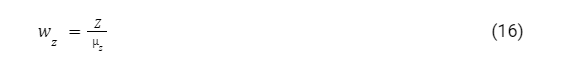
Where µz is the mean of the Z-Score of the dataset. Similarly, we have: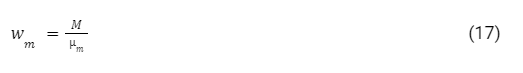
Where µm: the mean of the M-Score of the dataset.
- Assumption on the mean:
- In reality, we believe that the most of companies do not manipulate financial reports.
- The chosen dataset has to be well chosen with enough companies. It is preferable to get those companies from the same sector.
- Each mean is strictly in the green zone, so µz> 2.99 and µm < 2.22
- Features Decision Value for problematic cases
- In the case of F4 and F5, if wz > 1, F4 = 1 and F5 = 1, otherwise F4 = 0 and F5 = 0.
- In the case of F6 and F7, if wm is 1, then F6 = 1 and F7 = 1, otherwise F6 = 0 and F7 = 0.
These simple assumptions solve the problem of contradiction and use the mean metric of the whole dataset for comparison, which is more realistic for benchmarking.
- Decision variable and label for the model. All added features are Boolean and mutually exclusive. Let’s model the features as a matrix of features in 2 dimensions. M, Mij is a value where i represents the lines and j represents the columns. M can be divided into two matrices, S and F. Where S is the Score Matrix and F the Dummies’ feature matrix
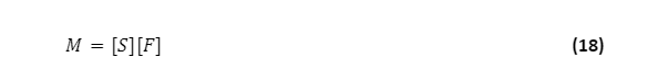
S=ZM Z and M are one column matrix with the respective values of Z-Score and M-Score.
. F=F1F2F3F4F5F6F7 Fi with i∈1..7 is a one column matrix with either 0 or 1 value
Let’s call D the one column decision matrix D is done by the logical OR operation on all Fi.
D=F1 OR F2 OR F3 OR F4 OR F5 OR F6 OR F7
Computation sample result of features
Table 4: Features
| Ticker | Z | M | F1 | F2 | F3 | F4 | F5 | F6 | F7 | D |
| AAPL | 4.997780081 | -2.84605607 | 1 | 0 | 0 | 0 | 0 | 0 | 0 | 1 |
| ACIW | 2.375941162 | -2.888564244 | 0 | 0 | 0 | 0 | 0 | 0 | 1 | 1 |
| ADI | 14.1561202 | -2.570731658 | 1 | 0 | 0 | 0 | 0 | 0 | 0 | 1 |
| ADP | 2.350243137 | -1.875429149 | 0 | 0 | 1 | 0 | 0 | 0 | 0 | 0 |
| ADSK | 8.939756358 | -2.780829754 | 1 | 0 | 0 | 0 | 0 | 0 | 0 | 1 |
| AMAT | 5.240279272 | -2.131774765 | 0 | 0 | 0 | 0 | 0 | 0 | 0 | 0 |
| AMKR | 0.464680878 | -3.199730753 | 0 | 0 | 0 | 0 | 0 | 1 | 0 | 1 |
| ASGN | 2.638839622 | -2.356403139 | 0 | 0 | 0 | 0 | 0 | 0 | 0 | 0 |
| AVGO | 13.50117851 | -2.727523123 | 1 | 0 | 0 | 0 | 0 | 0 | 0 | 1 |
| COMM | 0.552473697 | -2.264705123 | 0 | 0 | 0 | 0 | 0 | 0 | 0 | 0 |
| CSCO | 3.801959348 | -2.529372825 | 1 | 0 | 0 | 0 | 0 | 0 | 0 | 1 |
Feature Scaling and Dimension Reduction
Feature Scaling
It is recommended that they be rewritten at the same scale using standardization for improved model performance. We do not need to standardize Boolean features as F.
The result of standardization also called z scores, is that the features will be rescaled so that they’ll have the properties of a standard normal distribution with the mean = 0 and the standard deviation = 1. The standard score of a sample is calculated as follows:
Standardizing the features to make them centered around 0 with a standard deviation of 1 is essential when comparing measurements with different units; it is also a general requirement for the optimal performance of many machine learning algorithms.
Dimensionality Reduction
The primary purpose is to avoid overfitting and underfitting the model in the test data.
- Overfitting occurs when the model captures the patterns in the training data well but fails to generalize well to test data. Overfitting can happen when we have too many correlated features. In this case, the model has low bias and high variance.
- Underfitting happens when the model is not complex enough to capture the patterns in the training data well and, therefore, suffers from low performance on unseen data. In this case, the model has high bias and low variance.
Because all Fi in our study are linearly independent, and D is the result of the OR operation of all Fi, we can only keep Z and M as features, and D is the label column.
Table 5: Feature with scaling and dimensionality reduced
| Ticker | Z | M | D |
| AAPL | -0.0693653 | -0.50204105 | 1 |
| ACIW | -0.55669548 | -0.56680371 | 1 |
| ADI | 1.63292677 | -0.08257481 | 1 |
| ADP | -0.56147206 | 0.97674254 | 0 |
| ADSK | 0.66334334 | -0.4026665 | 1 |
| AMAT | -0.02429114 | 0.58619115 | 0 |
| AMKR | -0.91194798 | -1.04087662 | 1 |
| ASGN | -0.50782965 | 0.24396208 | 0 |
| AVGO | 1.51119051 | -0.32145201 | 1 |
| COMM | -0.89562963 | 0.38366717 | 0 |
| CSCO | -0.2916366 | -0.0195632 | 1 |
Processing model
The described model is processed with four different classifier algorithms to evaluate the best performing algorithm for our problem and select it for usage.
Classification result of the model
Figure 3: training dataset classification with four different algorithm

Figure 4: test dataset classification with four different algorithm

In these pictures, the blue zone (0) and the small blue square represent the companies that the model detected are engaging in fraud manipulation. In contrast the orange (1) and small triangles represent companies not found to be engaging in fraud manipulation.
Performance Analysis
Confusion Matrix and Score Overview
The confusion matrix (or error matrix) is one way to summarise the performance of a classifier for binary classification tasks. This square matrix consists of columns and rows that list the number of instances as absolute or relative “actual class” vs. “predicted class” ratios.
Let P be the label of class 1 and N be the label of a second class or the label of all classes not in class 1 in a multi-class setting.
Figure 5: Confusion Matrix definition

The score uses the confusion matrix result to return the ratio of accurate predictions. The formula does this ratio in percentage.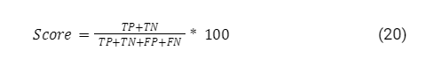
So, the higher the score, the better the model’s performance. The final appreciation is done in the test set to validate if the result is not misled by any problem such as overfitting or underfitting.
Table 6: Performance of the four classification algorithm on the model
| Classification Algorithms | Train | Test |
| Linear Regression | 90% | 86% |
| Support Vector Machine | 90% | 85% |
| Naïve Bayes | 90% | 57% |
| Decision Tree | 100% | 100% |
The general overview of the result shows that the feature selections were good, and there is no warning of overfitting or underfitting. The best performance is done by the decision tree classification algorithm, with 100% accuracy. So, at the end of this study, we choose the best-performing algorithm to build our model. In this case, it is the decision tree.
After building a model, the next step is to deploy it in production, but this phase is not part of this study. So, in production, if we want to classify one company, all we have to do is put the exact features of that company as input and then run the model to get the binary classification as an output.
Data Driven Research Theory
Mathematical models like Beinish’s M-Score and Altman’s Z-Score were initially made for one input. So those models are static; they don’t dynamically adapt their boundary decisions to the environment. Furthermore, financial statement behaviors can be different by industry sector, so it is essential to consider the dynamics of the industry to make a decision dynamically. One possible general approach for future research is redefining these models as follows.
Altman’s Z-Score and Beinish’s M-Score Probabilistic modeling
This model is also a probabilistic model, so we can assume that the model is following a normal distribution. So both models can be expressed as follows:
Standard Normal Distribution
The following formula calculates the Z score.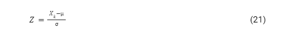
Where Xk is the standardized value, in this case, it is either the value of Altman’s Z-Score or Beinish M-score. With k=z for Altman’s Z-score and k= m for Beinish M-score.
µ is the mean of the distribution, as the standard deviation of the distribution
With this assumption, we see that dataset’s Altman Z-Score and Beneish M-Score can be expressed as a function of the mean and the standard deviation. In this approach, the mean and standard deviation are considered constant for the dataset, but they change for each dataset. Therefore, we hypothesize that the decision boundary in a data-driven can also be expressed in terms of the mean and the standard deviation. So the boundary limit should look like this:
Table 7: Data driven decision boundaries
| Safe Zone (green) | Intermediate Zone (yellow) | distress Zone (red) | |
| Altman’s Z-Score | Z ˃=ϕ(, µ ) | ψ(, µ )˂= Z ˂ ϕ(, µ ) | Z ˂ ψ(, µ ) |
| Beneish M-Score | M<= β(, µ ) | β(, µ )<M <= α(, µ ) | M >α(, µ ) |
This approach can be generalized to all kinds of models that are applied on entry and have a boundary decision constant. This opens a research area based on the experience of many datasets. The probabilistic model with the assumption of the normal distribution can be used as one research trail.
Conclusion
Altman’s Z-Score and Beinish’s M-Score are two proven financial reporting fraud, detection models. These models are based on mathematical formulas suitable for one company at a time. This study aimed to analyze one data-driven model using these two mathematical formulas as features and then build a new model of classification. We defined a new model that handles the problem of contradiction resulting from the two-based formulas. The problem we solved was a binary classification problem with a two-way decision on whether a company in the dataset is subject to financial manipulation or not. Ultimately, we trained and tested the model with four different algorithms, and the decision tree showed us better precision. In this case, the analysis of this data-driven model using a decision tree is our choice.
Author: William Tchoudi
Bibliography
[1] Beneish, Messod D. The Detection of Earnings Manipulation. Financial Analysts Journal, no. 5, Informa UK Limited, Sept. 1999, pp. 24–36. Crossref, doi:10.2469/faj.v55.n5.2296.
[2] Altman, E. (1968). Financial ratios. Discriminant analysis and the prediction of
corporate Bankruptcy. The Journal of Finance, Vol. 23(4), pp 589-609
[3] Muntari Mahama, Detecting Corporate Fraud And Financial Distress Using The Altman And Beneish Models, International Journal of Economics, Commerce and Management, UK, 2015
[4] Ganga Bhavani, Christian Tabi Amponsah, M-Score And Z-Score For Detection Of Accounting Fraud, Accountancy Business and the Public Interest 2017
 New Horizons in Education and Personal Development
LIGS University and ICAN Open Doors to Long-Term Success In today's dynamic…
 Relationship Management in the Oil and Gas Organizations: The Niger Delta Experience
No organization anywhere in the world could derive sustainable development without imbibing…
 How to write in academic style | APA 101
Writing an academic paper can be rough. There are so many rules…